Bayesian Bandits: Conjugate Priors for Bernoulli and Gaussian Arms
A policy that performs very well in a particular bandit may perform very poorly in another adversarially chosen bandit. In reality, the bandits are unknown. So, we need a policy that performs good in all bandits in average. If a policy that performs worse than another policy in at least one bandit and never performs better than the other policy in other bandits, then the first policy is said to be dominated by the second policy. A policy that isn’t dominated by any other policy is called an admissible or pareto optimal policy. There may be lots of admissible policies. One of them is the Minimax Optimal Policy that minimizes the worst regret across all bandits. It belongs to the following set:
Where, $R(\pi, \epsilon)$ is the regret of policy $\pi$ in bandit $v$. But this policy may have a high regret on average. So, let’s explicitly go for what we explicitly want. A policy that performs better on average than the others. The Bayesian optimal policy. When the environment $\epsilon$ is finite, it belongs to the following set:
Beta Distributions: Suppose, we tossed a coin 9 times. And the outcomes can be represented as a string E = “HTHHTHHHT”. If the probability of getting a head up is $p = x$, then the probability of this particular event is $x^{6}(1-x)^{3}$. The maximum likelihood estimate for $x$ should be $\frac{1}{3}$. And the likelihood that $Pr(p = x | E) = \frac{Pr(E|p = x) Pr(p = x)}{Pr(E)} = \frac{Pr(E|p = x) Pr(p = x)}{\int_{0}^{1} Pr(E|p = x) Pr(p = x) dx}$.
Initially, without any experiment, we can assume that, $Pr(p=x)$ is a uniform distribution for all values of $x$.
So,
It kind of makes sense, because the maximum likelihood estimate of $x$ will maximize the value of $Pr(p = x|E)$ which it should.
Now, We know that, $Pr(E | p = x) = x^{6} (1-x)^{3}$ but, we can replace E = “HTHHTHHHT” with a larger event called $\bar E = (a = 6, b = 3)$ where $a$ is the number of heads and $b$ is the number of tails. In that case,
So,
So,
Or more generally,
.
PDF of Beta Distribution: $f(x | \alpha, \beta) = \frac{x^{\alpha-1} (1-x)^{\beta-1}}{B(\alpha, \beta)}$ for all $0 \leq x \leq 1, \alpha > 0, \beta > 0$.
Mean: $\mu = \frac{\alpha}{\alpha + \beta}$
Variance: $\sigma^{2} = \frac{\alpha\beta}{(\alpha + \beta)^{2}(\alpha + \beta + 1)}$
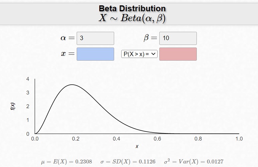
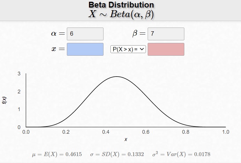
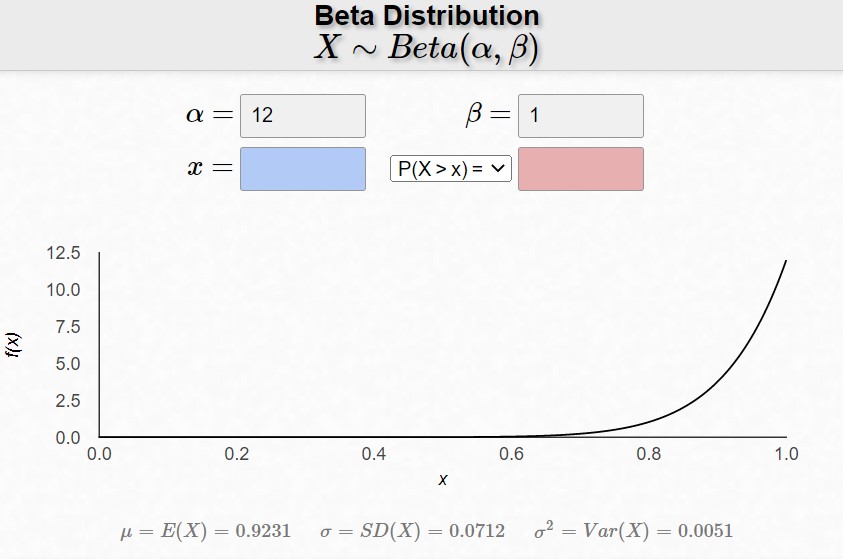
The above graphs show what happens when we change $\alpha$ by fixing $\alpha + \beta$. Notice that the graphs peak near $\frac{\alpha}{\alpha+\beta}$.
Conjugate Priors: Let’s say, we are conducting two coin-toss experiments. In the first experiment we got $\alpha$ heads and $\beta$ tails. And now, we are conducting the second experiment and we got $\gamma$ heads and $\delta$ tails. We want to update the probabilities of getting heads. Let’s call $E = (\gamma, \delta)$ the second experiment. We are interested in the following:
If $\bar E = (\alpha, \beta)$ was the first experiement, then $Pr(p = x) = Pr(p = x | \bar E)$. So, our posterior from the first experiment becomes the prior in the second experiment. So, $Pr(p = x) = \frac{x^{\alpha} (1-x)^{\beta}}{B(\alpha+1, \beta+1)}$. And if we plug it in,
Which is also a beta distribution. If the prior and posterior are of the same distribution family, then the prior is called a conjugate prior.
Bayesianism vs Frequentism: The main difference between Bayesian and Frequentist philosophy is that in Bayesian statistics, even if 3 heads came up during 10 coin tosses, any probability from 0 to 1 is plausible. Even though, $\frac{3}{10}$ will have the maximum likelihood, $\frac{1}{2}$ too will have some non-zero likelihood. But in the case of the Frequentist perspective, we are $100\%$ sure that the probability of getting a head is $0.3$. Also, Frequentist statistics doesn’t incorporate beliefs from previous experiments as priors unlike Bayesian statistics.
Bernoulli Arms: Suppose, we are showing ads to users. Ad number 1 was shown $\alpha + \beta$ times to people. It was clicked $\alpha$ times. In this situation, the reward is binary. Click or no click. In this case, every ad is a Bernoulli action/arm. And the Beta distribution captures this information so well. An appropriate prior distribution for this kind of arms is the Beta distribution.
Gaussian Arms: Most of the time, rewards of the arms aren’t binary. They are most of the time continuously valued having an unknown mean and an estimated worst case variance. In these situations, we assume that all the arms’ rewards are normally distributed around a carefully picked mean, with a large variance. Normal distributions too can be conjugate priors. Let’s say, the prior mean for such an arm is $\mu$ and prior variance is $\sigma^{2}$, and then utilize this arm $t$ and the arm reveals rewards, $x_{1}, x_{2}, x_{3}, \cdots, x_{t}$, then the posterior mean and variance will be,