MDPs: Markov Chains, Reducibility, Steady State Probabilities

Markov Chain: A Markov chain is a (possibly infinite) sequence of states of an environment where the transition from one state to another is stochastic and this transition probability only depends on the current state. The set of all possible states could be countably infinite. In the Discrete-Time Markov Chain, the transition from one state to another is a discrete event. In the Continuous-Time Markov Chain, at any given moment the environment is changing from one state to another. Let’s consider the following discrete example. For simplicity, we only assume that, there is only one type of weather possible for each day. Let’s say, there are only three types of weather. And any day can be classified to only one of those. The following diagram shows the state transition probability for each weather type.

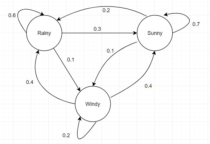
From this diagram, we can compute the probability of the following sequence of weather type: (sunny, sunny, windy, rainy, sunny) or in short (s, s, w, r, s). But how?

Stochastic Matrix: A right stochastic matrix is a square matrix where all of the entries are non-negative and the sum of each row is 1. Every stochastic matrix represents a finite markov chain. For example, the above state transition diagram can be expressed as a right stochastic matrix like this:

Also, a left stochastic matrix is one where the rows sum to 1 and a doubly stochastic matrix is both left stochastic and right stochastic.

Markov Assumption: A Markov Chain adheres to the Markov assumption that, the probably of the next state depends only on the current state. More formally,

Which can be succintly written as,

Time Homogeneity Assumption: We also assume that, the conditional state transition probabilities do not change over time. In other words,

So, using probability chain rule,

Now, applying the markov assumption here, we get,

Almost all of the quantities on the right can be immediately found from the above diagram. But how to find $p(S_{1} = s)$? This initial probability distribution among the starting states is problem dependent. Let’s say, $v_{0}$ is an $n\times 1$ vector so that $v_{0,i}$ is the probability that state $i$ is the initial state. So, $v_{n} = A v_{n-1}$, which yields $v_{n} = A^{n} v_{0}$.

Steady State: For most of the stochastic matrices, it turns out that, if $n$ is sufficiently large, then $v_{n+1} = v_{n}$ regardless of the initial probabilities. Since, $v_{n+1} = A v_{n}$, let’s say these vectors converge to another vector $v$, then $v = Av$. So, $v$ is an eigenvector of the eigenvalue 1. We will see that, for some special stochastic matrices we have a unique such vector $v$ which is called the steady state vector.

Reducibility: A Markov Chain is irreducible if any state can be reached from any state with some non-zero probability. And a Markov Chain is reducible if it’s not irreducible. An irreducible Markov Chain is also called strongly connnected in graph theoretic terminology.

Periodicity: A Markov Chain is periodic if there exists a $t > 1$ for which there exists a state $s$ so that $s$ can only be visited at time steps $t, 2t, 3t, \cdots $. A Markov Chain is aperiodic if every state can be visited at all time steps. In other words, for all states, the period $t = 1$.
Steady State Theorem: If a stochastic matrix is irreducible and aperiodic, then there exists a unique steady state vector which is it’s unit eigenvector for eigenvalue 1.

Since, $\lim_{n \to \infty} v_{n+1} = v_{n}$, therefore, $\lim_{n \to \infty} A^{n+1}v_{0} = A^{n}v_{0}$, and as $v_{0} \neq 0$, so, $\lim_{n \to \infty} A^{n+1} = A^{n}$. Which means, $A^{n}$ too converges. We can easily notice that $A^{n}[i][j]$ represents the probability of ending up at $j$ from state $i$ through some random walk of length $n$. This probability converges to a constant value. And we can also see that, $\lim_{n \to \infty} A^{n}[i][j] = A^{n}[k][j]$ for $i \neq k$. Which means all of the rows of that matrix are the same. And that tells us that the probability of ending up at state $j$ after a sufficiently long random walk doesn’t depend on the starting state. So, this row vector is just the same as $\lim_{n \to \infty} v_{n}$.