Contextual Bandits: A Literature Review
Here in this post, I will provide excerpts from some of the most influential works done on Contextual Multi-Armed Bandits.
Notation: $T$ is the horizon. $K$ is the number of arms. $\mathcal{M}$ is the set of policies.
2002: The Exp4 Algorithm by Auer et al The Exp4 algorithm can be perfectly used for the contextual bandit setting.
-
Problem setting:
- The bandit is adversarial.
- The environment is partially observable.
-
Regret Bounds:
- The upper bound for the expected regret is $\mathcal{O}(\sqrt{TK\log{M}})$.
-
Drawbacks and Scope of Improvement:
- The runtime is linear in $M$ in every round.
- The expected regret is quite good. But due to high variance, there is no guarantee that the regret stays concentrated around it's mean.
2007: The Epoch-Greedy Algorithm for Multi-armed Bandits with Side Information by Langford et al.
- Problem Setting:
- The environment is partially observable. You can only observe the reward for the arm you have chosen.
- The bandit is stochastic.
- Key Properties:
- Exploration and Exploitation rounds are distinct from each other. In the exploration round, they pull an arm uniformly at random and use the arm's reward to learn about the bandit. But in the exploitation step, the reward collected from the best arm suggested by the algorithm is ignored.
- In the exploration step, their goal is not to maximize immediate reward but in exploitation step, it is.
- The reward of an unexplored arm in a round is estimated by an Inverse-Propensity-Score.
- Makes no assumption about the time horizon $T$. As, in the stochastic scenario, if $T$ is known before hands, then it is better to always perform all the exploration steps first and then do all the exploitation steps. Likewise, here they spread this idea of exploration first and then exploitation to multiple epoch. At the beginning of each epoch, they explore one arm at random. Then if the average regret per round in the previous rounds is $\epsilon$, then they perform ${\left\lceil \frac{1}{\epsilon}\right\rceil}$ exploitation steps per epoch.
- Compares regret relative to the total reward of the best hypothesis.
- Regret Bound:
- The worst case regret bound for epoch greedy is $\mathcal{O}(T^{\frac{2}{3}} (K \log{M})^{\frac{1}{3}})$ where $T$ is the time horizon, $K$ is the number of arms and $M$ is the size of the hypotheses class.
- Drawbacks and Scope of Improvement:
- Compared to $Exp4$, has better regret bound dependence on $\log{M}$ and $K$ but worse dependence on $T$.
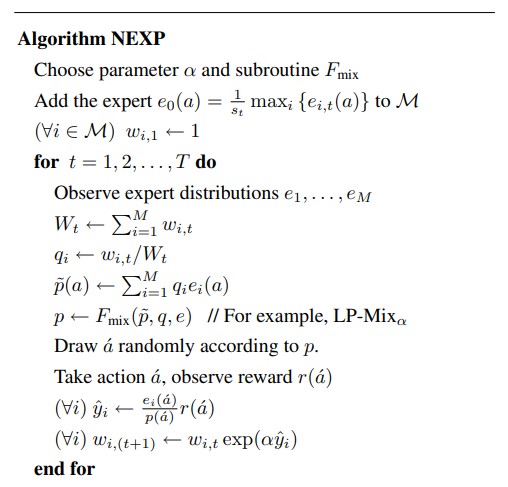
2009: NEXP Algorithm by McMahan et al.
-
Problem Setting:
- The bandit is non-stochastic.
- The environment is partially observable.
-
Key Properties:
- Compares regret relative to the expected reward obtained by the best expert.
- Uses the fact that when $K$ is significantly large and even larger than $M$, then the regret upper bound need not be $\sqrt{TK \log{M}}$.
- Official Pseudocode:
-
They have proposed several variants of the $F_{mix}$ subroutine. One of them is $UA_{mix}(\lambda)$:
$p(a) = (1-\lambda) \bar p(a) + \lambda \frac{1}{K}$ where $\lambda$ is an egalitarianism factor
-
Another variant of $F_{mix}$ is $UE_{mix}(\lambda)$:
$p(a) = (1-\lambda) \bar p(a) + \frac{\lambda}{M} \sum_{i}^{} e_{i}(a)$ -
Yet, another variant is called $LP_{mix}(\alpha)$:
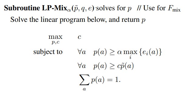
- Regret Bounds:
- When they use the $UA_{mix}$ subroutine, the expected regret is bounded from above by $E[R] \leq 2.63 \sqrt{TM \log{M}}$.
- When they use the $LP_{mix}$ subroutine, the expected regret is bounded from above by $E[R] \leq 2.63 \sqrt{TS \log{M}}$ where $S \leq min(K,M)$.
-
Drawbacks and Scope of Work::
- The runtime complexity in each round is $\mathcal{|A|+|M|}$.
2011: The Exp4.p Algorithm by Beygelzimer et al
-
Problem setting:
- The bandit is adversarial.
- The environment is partially observable.
- Makes the assumption that $\log{M} \leq TK$.
-
Regret Bounds:
- With probability at least $1-\delta$, expected regret is bounded by $\mathcal{O}(\sqrt{TK\log{\frac{M}{\delta}}})$.
- With high probability, the algorithm guarantees that the upper bound for the expected regret is $\mathcal{O}(\sqrt{TK\log{M}})$.
- In the stochastic scenario, even if the policy class may be of an infinite size but if it has a finite VC dimension $d$, then the algorithm guarantees with high probability that the expected regret is bounded by $\mathcal{O}(\sqrt{Td\log{T}})$.
-
Drawbacks and Scope of Improvement:
- Like it's predecessor $Exp4$, the runtime is linear in $M$ in every round.
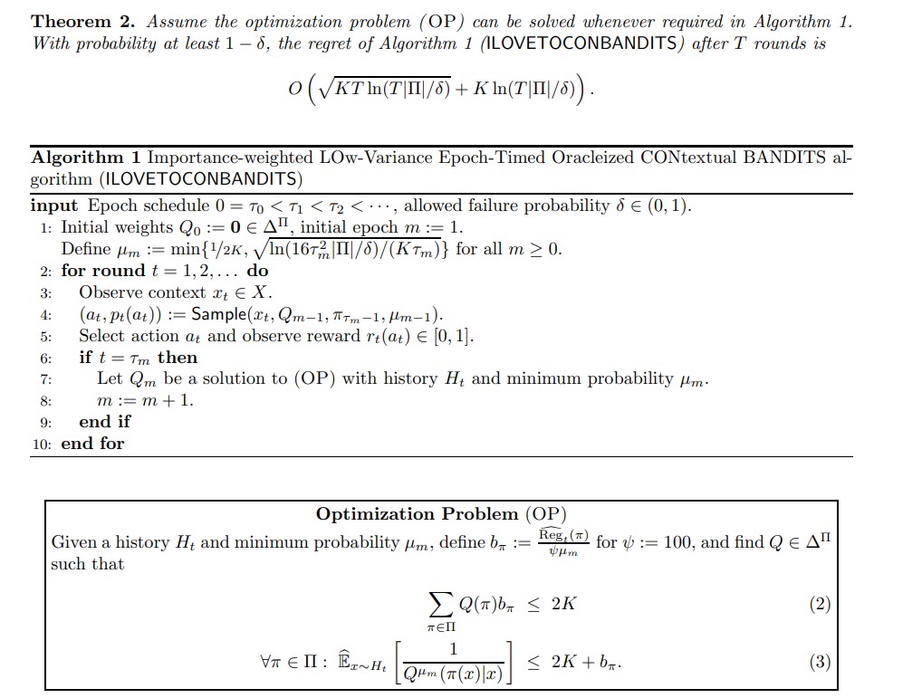
2014: ILOVETOCONBANDITS: Taming the Monster by Agarwal and Schapire et al
-
Problem Setting:
- The bandit is stochastic.
- We can only observe the reward for the action chosen.
-
Key Properties:
- They use inverse propensity score to estimate the reward at round $t$ if they chose action $a$ given the history $H_{t-1} = (C_{1}, A_{1}, X_{1}, C_{2}, A_{2}, X_{2}, \cdots, C_{t-1}, A_{t-1}, X_{t-1})$.
- They have access to an Oracle that returns the policy that maximizes the total reward in the first $t-1$ rounds according to this estimated reward system.
- Compares regret relative to the expected reward obtained by the best policy.
- The algorithm calculates a distribution over the policy space. Then randomly samples a policy from that space. This policy also is a probability distribution over the actions. Then the algorithm chooses an action at random.
- Since they use the inverse propensity score to estimate the rewards, if the probability of an action being chosen at round $t$ is very low, then it induces a large variance on the reward estimate. So, they don't allow any of that probabilty to become less than $\mu \in [0, \frac{1}{K}]$.
- Unlike it's precursors such as Randomized UCB, this algorithm doesn't call the oracle in every round. It uses a epoch schedule like the doubling trick and calls the oracle only at the beginning of the epoch
- If $\tau_{m}$ is the current epoch schedule and $\tau_{m+1}$ is the next epoch schedule, then $\tau_{m+1} \leq 2\tau_{m}$
- Uses coordinate descent to solve the optimization problem
- Makes only $\sqrt{\frac{KT}{\log{\frac{\mathcal{M}}{\delta}}}}$ calls to the oracle which is phenomenal compared to it's precursor Randomized UCB
- Official Pseudocode:
- Regret Bounds:
- Their algorithm gives optimal regret: $\mathcal{O}(\sqrt{TK\log{\frac{T\mathcal{M}}{\delta}}})$ with confidence at least $1-\delta$.
-
Drawbacks and Scope of Work::
- Time complexity is $\sqrt{\frac{K^{3}T^{3}}{\log{\frac{\mathcal{M}}{\delta}}}}$. Can be optimized.
- The oracle is an offline regressor which prossesses batches of data at the start of each epoch. So, at the end of the end, the algorithm kind of uses stale knowledge about the environment.
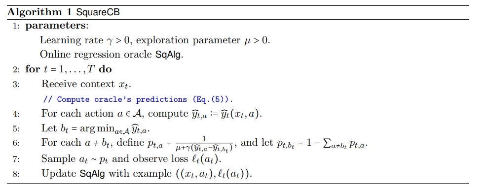
2020: Beyond UCB: SquareCB by Dylan Foster and Alexander Rakhlin
-
Problem Setting:
- Makes no assumption about the bandit environment.
- We can only observe the reward for the action chosen.
-
Key Properties:
- Oracle based algorithms compute a distribution over all the policies. Then they randomly sample a policy from that distribution. And that policy is also a distribution across arms. Then they randomly sample an arm. So, this distribution across policies is a middleman. We can get rid of that. The authors keep a single online regressor oracle that estimates the expected reward of each arm. Then chooses the best arm.
- Now, this may feel like choosing the arm is deterministic. How can we allow exploration then?
- Any arm whose estimated reward is deviated from that of the best arm has less likelihood of being chosen. They create a probability distribution in the following way
- Let $\bar y_{t,a}$ be the estimated reward of arm $a$ at round $t$. And let $b_{t}$ be the best arm mentioned above. Then for all other arms, $p_{t,a} = \frac{1}{\mu + \lambda (\bar y_{t,b_{t}} - \bar y_{t,a})}$ and for $b_{t}$, $p_{t,b_{t}} = 1 - \sum_{a \neq b_{t}}^{} p_{t,a}$. This is inspired from an old paper of Abe and Long.
- This is $\mu$ is the exploration factor. It's the same for everyone and $\lambda$ is the learning rate.
- Then the action is randomly sampled from this distribution.
- Official Pseudocode:
- Regret Bounds:
- Their algorithm gives optimal regret: $\mathcal{O}(\sqrt{TK\log{\mathcal{M}}})$ for finite classes $\mathcal{M}$.
- If the regression oracle is an online least square linear regressor, then the regret is $\mathcal{O}(\sqrt{TKd})$ where $d$ is the dimension of the context space.
- If the regression oracle is an online gradient descent linear regressor, then the regret is $\mathcal{O}(\sqrt{TK\sqrt{T}})$.
-
Drawbacks and Scope of Work::
- The Algorithm uses an online regression oracle. There is no algorithm yet that uses an online classification oracle.