ML Theory: Linear Models

Regression: Regression is the task of estimating the value of one variable that’s dependent on other variables. For example: determining the rent of a house is a function of the area of the house by square feet, the number of bedrooms, location and other facilities and the salary of a person is a function of his educational background and skill-set etc. There are lots of regression models. We will discuss only the linear model here. But the best in practice are Kernel Ridge regression, Support Vector regression, Lasso etc.

Multivariate Linear Regression Imagine that the features of a house can be numerically expressed as the following vector $x = (x_{1}, x_{2}, \cdots, x_{n})$ where $x_{1}$ can mean the number of kitchen or $x_{2}$ can mean whether there is a gym in the building or not. In problems where a change in the indepdendent variables lead to a linear change in the dependent variables, linear regression is a perfect solution. Our linear hypothesis is that if $y$ is the house rent, then,

$y = h_{w}(x) = w_{1} x_{1} + w_{2} x_{2} + \cdots + w_{n} x_{n} + w_{n+1}$

So, if we extend the vector $x$ by one dimension by appending a dummy 1 at the end $x = (x_{1}, x_{2}, \cdots, x_{n}, 1)$, we can express $y$ as follows,

$y = w^{T}x = x^{T}w$

Where $w = (w_{1}, w_{2}, \cdots, w_{n}, w_{n+1})$
So, if we are given $m$ data points $(x^{(1)}, y^{(1)}),(x^{(2)}, y^{(2)}),\cdots, (x^{(m)}, y^{(m)})$, the squared error should be:

$ E = \sum_{i=1}^{m} (y^{(i)} - (x^{(i)})^{T}w)^{2}$

We can express the above equation in the following matrix form:

$E(W) = ||Y - X^{T}W||^{2}$

Where,

$Y = \begin{bmatrix}y^{(1)}\\y^{(2)}\\.\\y^{(m)}\\\end{bmatrix}, X = \begin{bmatrix}x^{(1)}_{1} & x^{(2)}_{1} & . & x^{(m)}_{1}\\ x^{(1)}_{2} & x^{(2)}_{2} & . & x^{(m)}_{2}\\ . & . & . & .\\ x^{(1)}_{n+1} & x^{(2)}_{n+1} & . & x^{(m)}_{n+1}\\\end{bmatrix}, W = \begin{bmatrix}w_{1}\\w_{2}\\.\\w_{n+1}\\\end{bmatrix}$

We want to solve for a $W$ so that the error is minimized. Since $E$ is convex and differentiable, it admits a global minimum at a certain $W$ where $\nabla E(W) = 0$. In other words,

$2X(X^{T}W - Y) = 0$ $XX^{T}W = XY$

If $XX^{T}$ is invertible, then there is a unique solution, $W = (XX^{T})^{-1}XY$. Otherwise, we can get a family of solutions,

$W = (XX^{T})^{+}XY + (\mathcal{I} - (XX^{T})^{+}XX^{T})A$

where $A$ is an arbitrary matrix and $(XX^{T})^{+}$ is the Moore-Penrose Pseudo-Inverse of $XX^{T}$. The solution with the smallest norm is achieved when $A = 0$.
The overall complexity of the solution is $\mathcal{O}((m+n)n^{2})$.

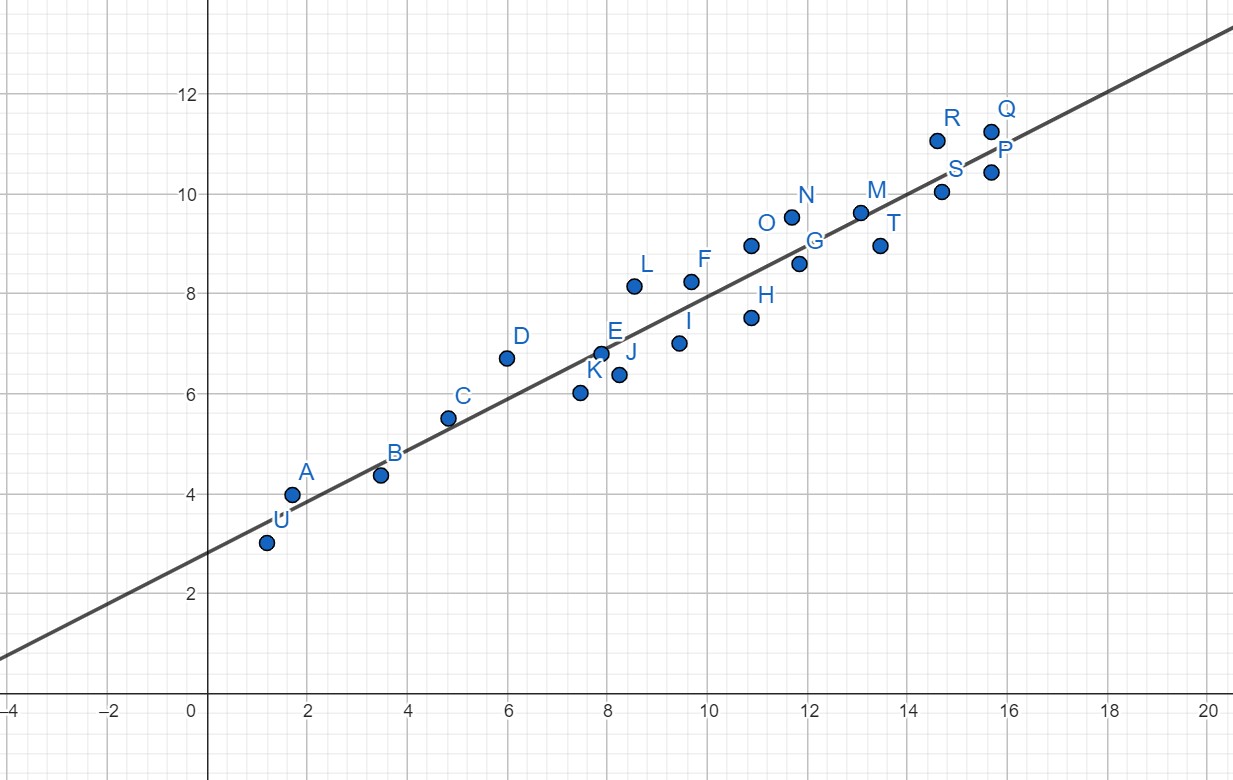
Univariate Linear Regression: Let’s say, we only have one feature. So, our linear hypothesis is very simple.

$h_{w}(x) = w_{1}x + w_{2}$

So, the loss over the whole data set can be formulated as,

$E(W) = \sum_{i = 1}^{m} (y_{i} - (w_{1} x_{i} + w_{2}))^{2}$

We want to find values of $w_{1}$ and $w_{2}$ so that $E$ is minimized. That will happen when $\frac{\partial E}{\partial w_{1}} = 0$ and $\frac{\partial E}{\partial w_{2}} = 0$. These two equations lead to,

$2 \sum_{i=1}^{m} (y_{i} - (w_{1} x_{i} + w_{2})) x_{i} = 0$ $2 \sum_{i=1}^{m} (y_{i} - (w_{1} x_{i} + w_{2})) = 0$

Here, we have two equations with two variables.

$w_{1} \sum_{i= 1}^{m} x_{i}^{2} + w_{2} \sum_{i=1}^{m} x_{i} = \sum_{i=1}^{m} x_{i}y_{i}$ $w_{1} \sum_{i= 1}^{m} x_{i} + w_{2} \sum_{i=1}^{m} 1 = \sum_{i=1}^{m} y_{i}$

Solving for $w_{1}$ and $w_{2}$ yields,

$w_{1} = \frac{m(\sum_{i=1}^{m}x_{i}y_{i}) - (\sum_{i=1}^{m}x_{i}) (\sum_{i=1}^{m}y_{i})}{m(\sum_{i=1}^{m}x_{i}^{2}) - (\sum_{i=1}^{m}x_{i})^{2}}, w_{2} = \frac{(\sum_{i=1}^{m}x_{i}^{2})(\sum_{i=1}^{m}y_{i}) - (\sum_{i=1}^{m}x_{i}) (\sum_{i=1}^{m}x_{i}y_{i})}{m(\sum_{i=1}^{m}x_{i}^{2}) - (\sum_{i=1}^{m}x_{i})^{2}}$

Linear Regression with Learning: When your dataset is constantly changing, new data are coming in, we can’t use the above approach of solving a system of linear equations. But we can use gradient descent to learn better values of the weights. The weight update rule should look like this:

$w_{i} = w_{i} - \lambda \frac{\partial E}{\partial w_{i}}$

Where $\lambda$ is the learning rate. In the case of the univariate linear regression model,

$w_{1} = w_{1} + \lambda \sum_{i=1}^{m}(y_{i} - h_{w}(x_{i}))x_{i}$ $w_{2} = w_{2} + \lambda \sum_{i=1}^{m}(y_{i} - h_{w}(x_{i}))$

The above approach is called batch gradient descent because while calculating the error we are using the whole dataset. In this case, convergence to the global minimum is guaranteed if we take $\lambda$ small enough. But the algorithm is very slow. In each step of the iteration for all data points we have to compute $h_{w}(x)$ because the weights are being updated in each iteration. We need to use the updated values of weights in the next iteration. The complexity of this approach is $\mathcal{O}(kmn)$ where $k$ is the number of iterations which is a function of $\lambda$ and the dataset, $m$ is the size of the dataset and $n$ is the dimension of the feature space.

There is another approach called stochastic gradient descent where in each iteration of the algorithm, we don’t use the whole dataset to compute the error. We only randomly select one data point to compute the error. This way, the iterations are faster. So SGD is much faster than BGD. But the problem is with a fixed $\lambda$, the algorithm keeps on going back and forth over the global minimum choices of the weights instead of settling down. But with a monotonously decreasing series of $\lambda$, SGD reaches the global minimum.

Batch gradient descent is slow. Stochastic gradient descent is spurious and can induce bias. A middle ground is mini-batch gradient descent. Instead of sampling one data point per iteration, we can sample 200-500 data points dependending on the problem instance.

Classification using Linear Regression: If two sets of n-dimensional points are separable by a hyperplane, then we can use linear regression and hard threshold to classify those points. In the diagram given below, the 2-D points can be separated with a line and thus we can use linear regression to learn such a decision boundary.
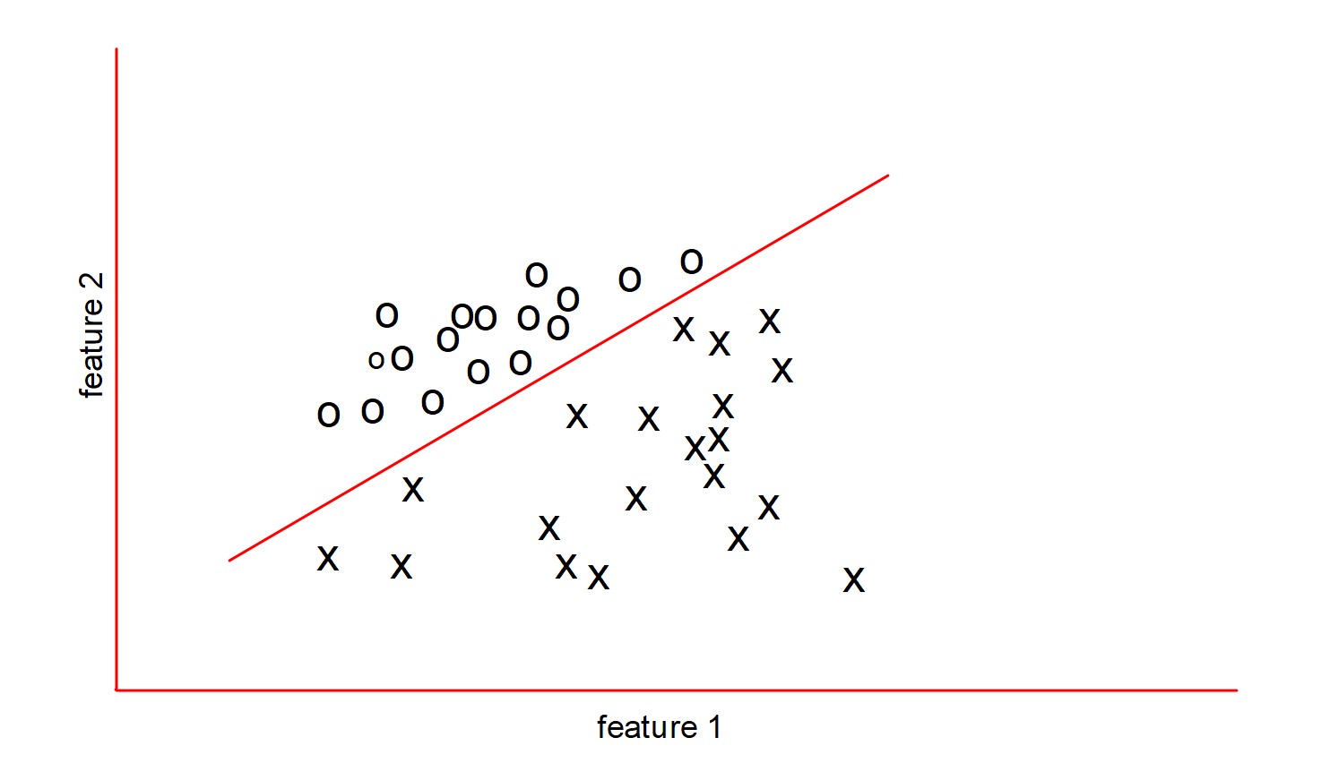
Let’s say we are trying to classify the above points as “good” and “bad”. We will express them as +1 and -1 respectively. Then our hypothesis will be:

$h_{w}(x) = sign(w_{1} x_{1} + w_{2} x_{2} + w_{3})$

But how to define error in this case? If we define the error as the total number of misclassification, then the error function doesn’t remain a continuous and differentiable function. However, an update rule of the following form works:

$w_{i} = w_{i} + \lambda \sum_{j=1}^{m}(y^{(j)} - h_{w}(x^{(j)}))x^{(j)}_{i}$

Classification using Logistic Regression: The hard threshold function is not continuous and differentiable. To make learning a more predictable endeavour, we can use the logistic function to determine the probability that our output is 1 given that we are trying to classify points into the class $\{0, 1\}$.

$L(h_{w}(x)) = \frac{1}{1 + e^{-h_{w}(x)}}$

Then we can use the squared loss and get the following update rule:

$w_{i} = w_{i} + \lambda \sum_{j=1}^{m}(y^{(j)} − h_{w}(x^{(j)}))h_{w}(x^{(j)})(1 − h_{w}(x^{(j)}))x^{(j)}_{i}$

A better loss function is the Shannon Entropy when $y^{(i)} \in \{-1, 0\}$:

$\sum_{i=1}^{m}-y^{(i)} \log{(L(h_{w}(x^{(i)})))} -(1-y^{(i)}) \log{(1 - L(h_{w}(x^{(i)})))}$

Another loss function can be when $y^{(i)} \in \{-1, +1\}$:

$\sum_{i=1}^{m}\log{(1 + e^{-y^{(i)}h_{w}(x^{(i)})})}$

Drawbacks:

The data may not be linearly separable.
It doesn't minimize the norm of the weight vector and thus can lead to increased solution complexity and overfitting. The objective to minimize should be: $\gamma ||W||^{2} + ||Y - X^{T}W||^{2}$ for some hyper-parameter $\gamma$.