MDPs: Markov Reward Model, Markov Decision Process, Bellman Equations

2022, Oct 01    

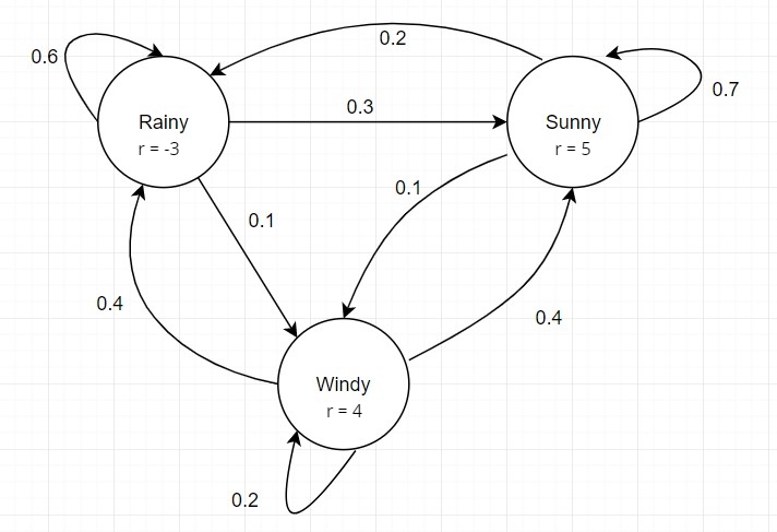
Markov Reward Model: A Markov chain was only a pair $\langle S, A\rangle$ where $S$ is the set of states and $A$ is the stochastic state transition matrix. From this information, we can only find out which states are more likely to occur on a random walk. But if we associate a reward with each state, then some states become more desirable than others. In this way, the Markov Reward Model can send some feedback to the agent. So, a Markov Reward Process/Model is a quadruple $\langle S, A, R, \gamma \rangle$ where $R$ is a function that maps each state to a reward, $R(S_{t}) = R_{t}$ and $\gamma$ is a discount factor which will be explained later.

Return: If $S_{0}, S_{1}, \cdots, S_{T}$ is a path/trajectory, then the return or gain of that path is the cumulative reward.

$G_{t = 0: T} = \sum_{t = 0}^{T} R(S_{t}) = \sum_{t = 0}^{T} R_{t}$

The goal of the agent is to walk a path before the time horizon $T$ so that, the total reward is maximized.

Discounted Return: Sometimes, to the agent, immediate rewards are more important than future ones. But the future rewards aren’t irrelevant either. Rather their importance is diminishing with time, rather than the other way round. One way to think of it is, if we prioritize distant rewards more than current rewards, the agent would be procrastinating. Tomorrow is more important than today and so we can slack off a bit. That way, the agent never gets much done. So, we introduce a $0 < \gamma \leq 1$.

$G_{t = 0: T} = \sum_{t = 0}^{T} \gamma^{t}R(S_{t}) = \sum_{t = 0}^{T} \gamma^{t}R_{t}$

One good thing about the discounted return is that it can allow $T$ to be infinite. In the case of the cumulative return, it might not even be a finite value. But with $\gamma$ less than 1, we can make the return converge. If $\gamma = 1$, then it’s just the old cumulative reward. But if $\gamma$ is very close to 0, then the agent is actually miopic ( short-sighted ) and only seeks to maximize per round reward.

Value Function: How good a state is in terms of being a starting state can be measured from the expected return from all possible trajectories of arbitrary lengths that start from that state. It’s called the value function of that state and it’s defined as:

$v(s) = \mathbb{E}[G_{t=0:\infty} | s_{0} = s] = \mathbb{E}[ \sum_{t = 0}^{\infty} \gamma^{t}R_{t} | s_{0} = s]$

Markov Decision Process: Markov Chains and Markov Reward Models don’t have any explicit notion of an action. Changing the state itself could be deemed as an action. And the reward was associated with next state. So, actions were deterministic. The actions were a mapping from one state to another. But we can decouple the definition of an action from just a mapping between states. An agent might choose action $a$ being at state $s$, but still remain uncertain about the identity of the next state. A Markov Decision Process(MDP) is a tuple $\langle S, A, P, R, \gamma \rangle$ where $P$ is a conditional probability distribution. $P(s^{‘}\vert s,a) = p(S_{t+1} = s^{‘} \vert S_{t} = s, A_{t} = a)$ means the probability of ending up at state $s^{‘}$ from state $s$ by taking action $a$. And the reward function also takes into account the current state and the current action. $R_{t} = R(S_{t}, A_{t})$.

Policy: A policy is a strategy of the agent. It’s the agent’s estimation of the profitability of an action from a particular state. $\pi(a|s)$ is a probability distribution across the actions from the state $s$. $\pi(a|s) = p(A_{t} = a | S_{t} = s)$.
Expected Return: The expected return of a policy is the expected return of any trajectory from any starting state by following that policy. It’s defined as follows,

$J(\pi) = \int_{\tau}^{} p(\tau|\pi) R(\tau)$

The optimal policy $\pi^{*}$ is one that belongs to the following set:

$\arg \max_{\pi} J(\pi)$

Value Function: Given a policy $\pi$, the value function of a state is the expected return of a trajectory starting from that state.

$v_{\pi}(s) = \mathbb{E}_{\tau \sim \pi}[R(\tau)|S_{0} = s]$

Action-Value Function: Given a policy $\pi$, the action-value function of an action-state pair is the expected return of a trajectory starting from that state and choosing that action.

$q_{\pi}(s, a) = \mathbb{E}_{\tau \sim \pi}[R(\tau)|S_{0} = s, A_{0} = a]$

Also note that,

$v_{\pi}(s) = \mathbb{E}_{a \sim \pi}[q_{\pi}(s,a)]$

Bellman Equations: One easily comes up with the following,

$q_{\pi}(s) = \mathbb{E}[ R_{0} + \gamma R_{1} + \gamma^{2} R_{2} + \cdots | S_{0} = s]$ $q_{\pi}(s) = \mathbb{E}_{a \sim \pi(.\vert s)}[ R_{0} + \gamma R_{1} + \gamma^{2} R_{2} + \cdots | S_{0} = s, A_{0} = a]$ $q_{\pi}(s) = \mathbb{E}_{a \sim \pi(.\vert s)}[ R_{0}] + \mathbb{E}_{a \sim \pi(.\vert s)}[\gamma R_{1} + \gamma^{2} R_{2} + \cdots | S_{0} = s, A_{0} = a]$ $q_{\pi}(s) = \mathbb{E}_{a \sim \pi(.\vert s)}[ R_{0}] + \sum_{s' \sim p(.\vert s, a) } p(s'\vert s, a ) \mathbb{E}_{a \sim \pi(.\vert s)}[\gamma R_{1} + \gamma^{2} R_{2} + \cdots | S_{1} = s']$ $q_{\pi}(s) = \mathbb{E}_{a \sim \pi(.\vert s)}[ R_{0}] + \gamma \sum_{s' \sim p(.\vert s, a) } p(s'\vert s, a ) v_{\pi}(s')$ $q_{\pi}(s) = \mathbb{E}_{a \sim \pi(.\vert s)}[ R_{0}] + \gamma \mathbb{E}_{a \sim \pi(.|s), s' \sim p(.|s,a)} [v_{\pi}(s')]$ $q_{\pi}(s) = \mathbb{E}_{a \sim \pi(.|s), s' \sim p(.|s,a)} [r + \gamma v_{\pi}(s')]$

Analogously, for the action-value function, one can guess and similarly derive the following:

$q_{\pi}(s, a) = \mathbb{E}_{s' \sim p(.|s,a), a' \sim \pi(. | s')} [r + \gamma q_{\pi}(s', a')]$

So, the value function vector is defined in term’s of itself, $v = r + \gamma Pv$. It can be solved from $v = (1-\gamma P)^{-1}r$ which takes $\mathcal{O}(n^{3})$ complexity. But we can use Monte Carlo simulation or Dynamic Programming to yeild faster solutions.

Optimal State-Value Function: For a state $s$, it’s maximum value across all policies is called $v_{*}(s)$.

$v_{*}(s) = \max_{\pi} v_{\pi}(s)$

Optimal Action-Value Function: For a state $s$ and an action $a$, the maximum action-value of this pair across all policies is called $v_{*}(s, a)$.

$q_{*}(s, a) = \max_{\pi} q_{\pi}(s, a)$ $q_{*}(s, a) = \mathbb{E}[R(s,a) + \gamma \max_{\pi} \mathbb{E}[q_{\pi}(s', a')]]$ $v_{*}(s) = \max_{a \sim A} q_{*}(s,a)$

Bellman Optimality Equations: The following equations are rather straightforward:

$v_{*}(s) = \max_{a} \mathbb{E}_{s' \sim p(.|s,a)} [R(s,a) + \gamma v_{*}(s')]$ $q_{*}(s,a) = \mathbb{E}_{s' \sim p(.|s,a)} [R(s,a) + \gamma \max_{a'} q_{*}(s', a')]$